Tests
frzout has a standard set of unit tests, whose current CI status is:

The unit tests do not check the model’s physical accuracy, which is difficult to verify automatically. Instead, this page shows a series of plots which can be quickly checked manually. Essentially, they are visual unit tests.
Each plot compares sampled quantities (colored lines) to expectations (dark grey lines). A test passes if the lines agree.
The remainder of this page is automatically generated by plot_tests.py in the frzout repository.
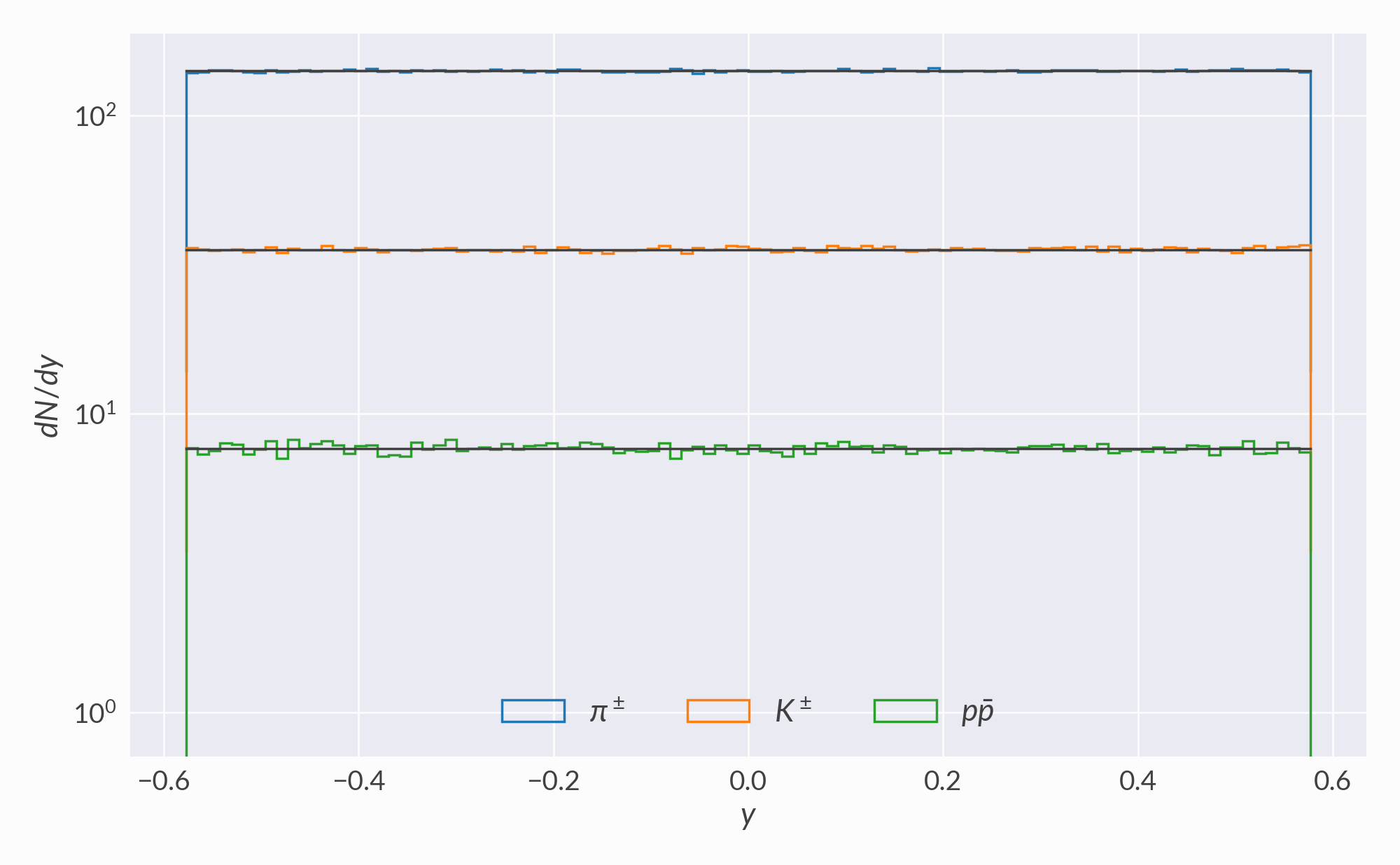
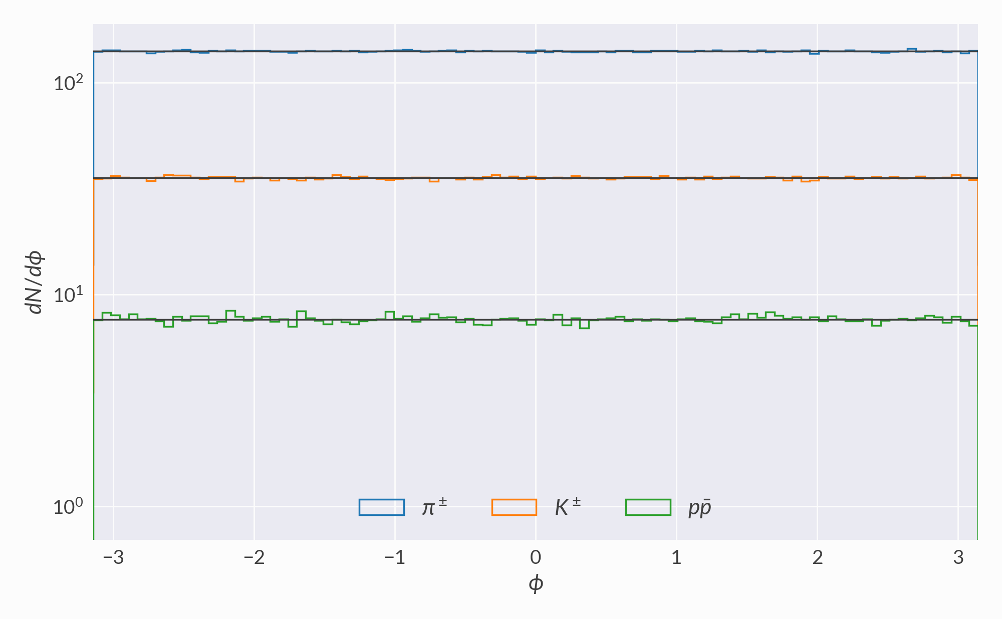
Stationary box
A single boost-invariant volume element with zero flow velocity. This is a rudimentary test case with easily-calculated observables.
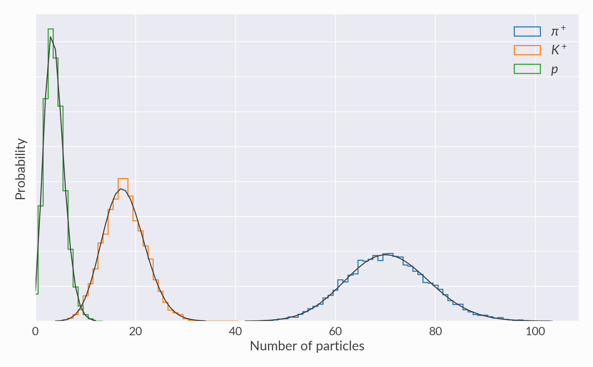
Multiplicity distributions
These are histograms of particle counts from many oversamples. Production of each species should be Poissonian:
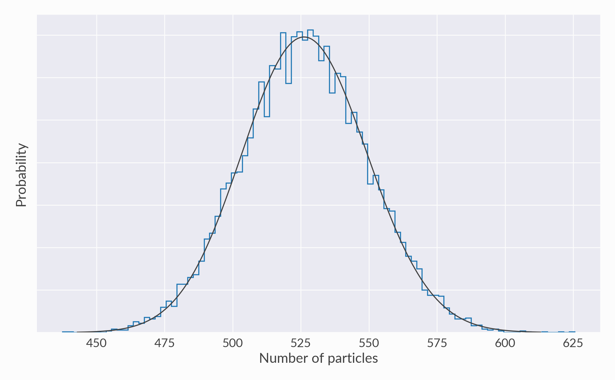
Overall particle production (all species) should also be Poissonian:
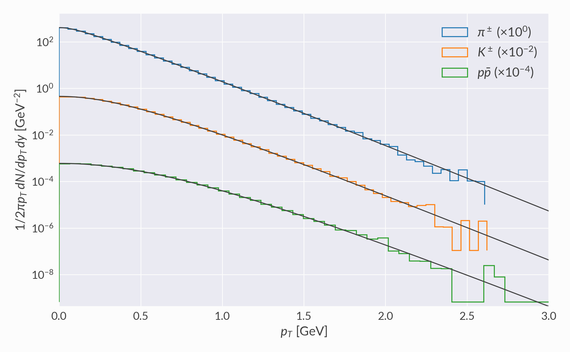
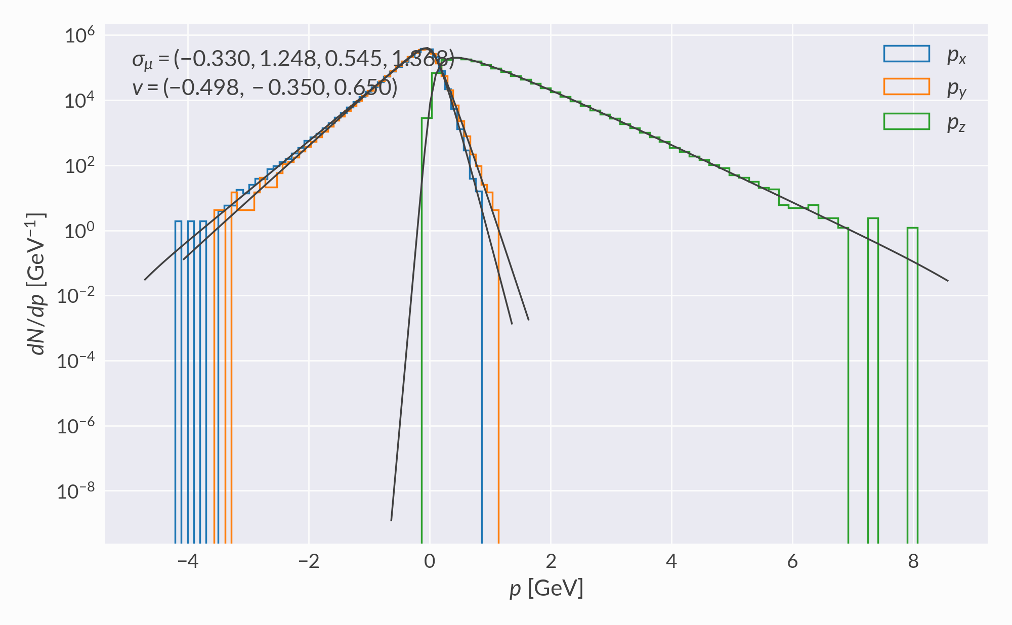
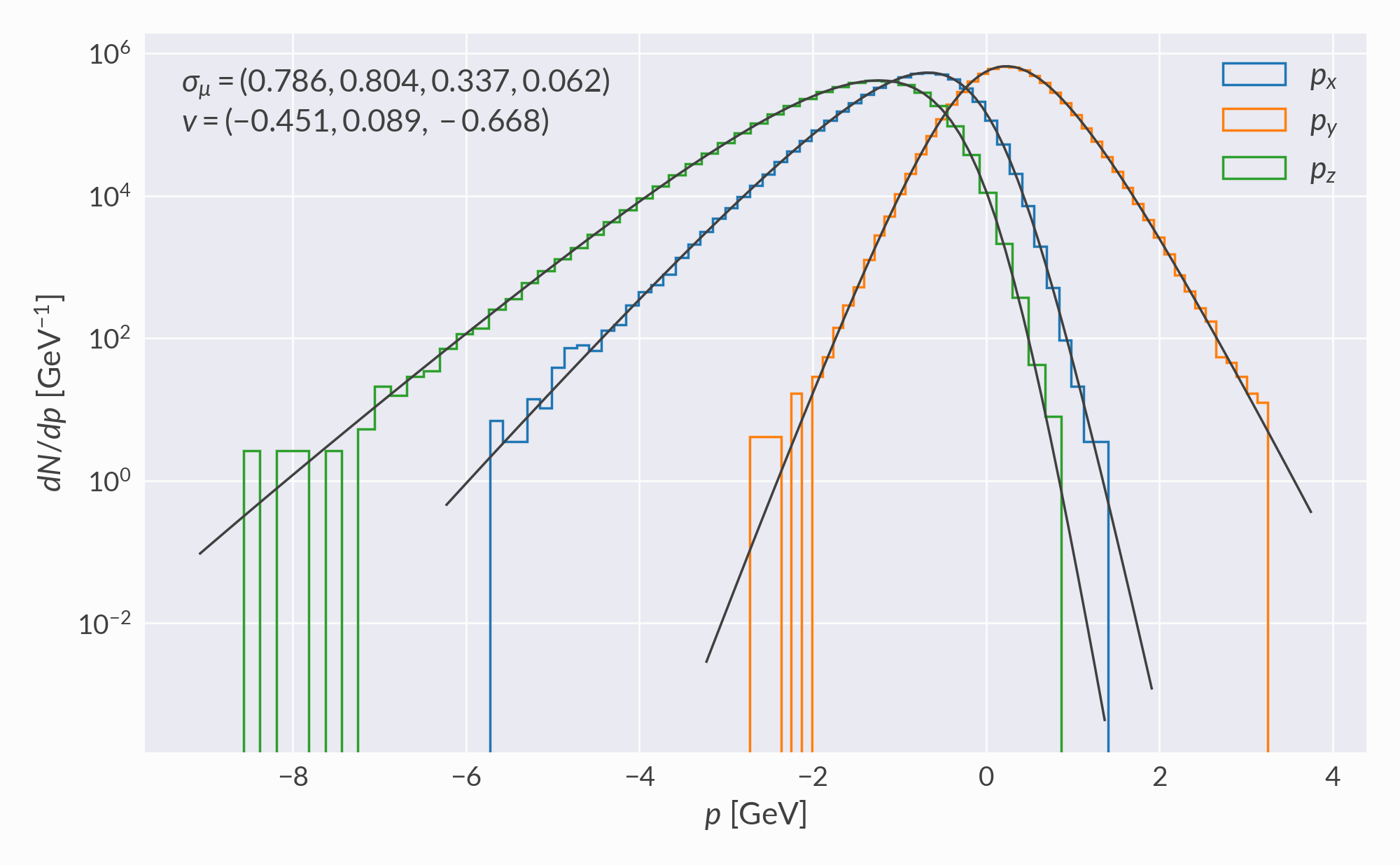
Moving box
A single 3D volume element with randomly chosen flow velocity and normal vector (this randomness means the volume element is not necessarily realistic for a heavy-ion collision, but it is still numerically valid).
Histograms of sampled (x, y, z) momenta are compared to distributions computed by numerically integrating the Cooper-Frye function. Negative contributions are ignored.
\(\pi^\pm\) momentum
\(K^\pm\) momentum
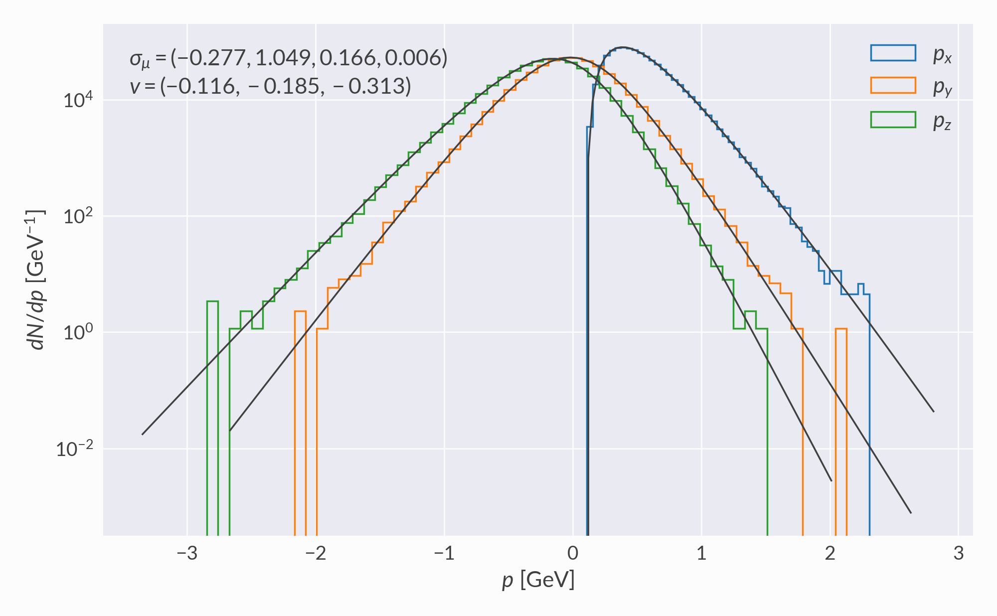
\(p \bar p\) momentum
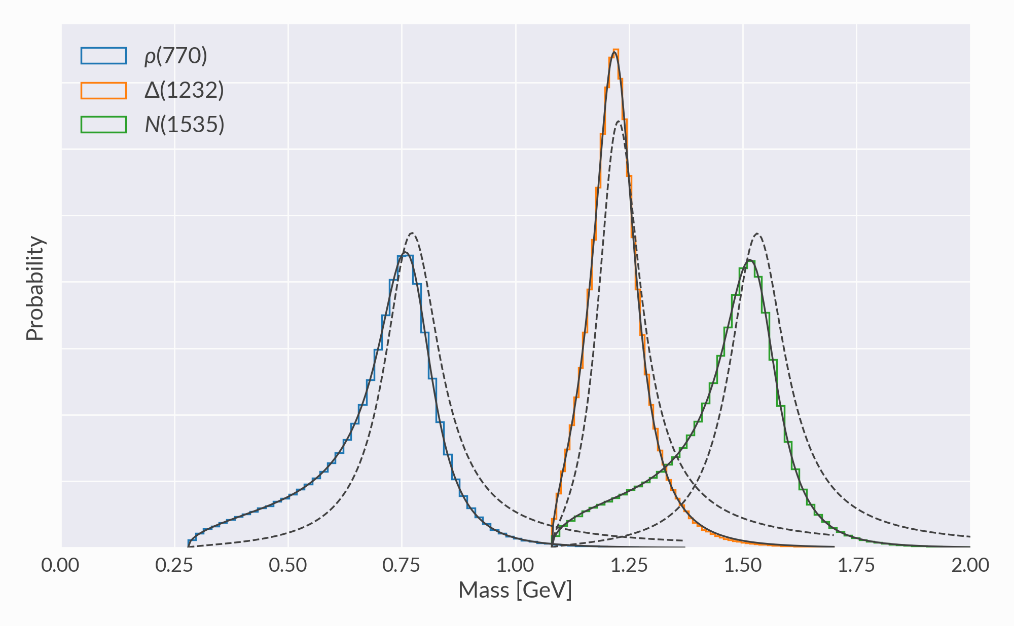
Resonance mass distributions
Verification of mass disributions for several resonance species. Grey dashed lines are the Breit-Wigner distributions with mass-dependent width, grey solid lines are the same distributions with momentum integrated out, and colored lines are histograms of the sampled masses.
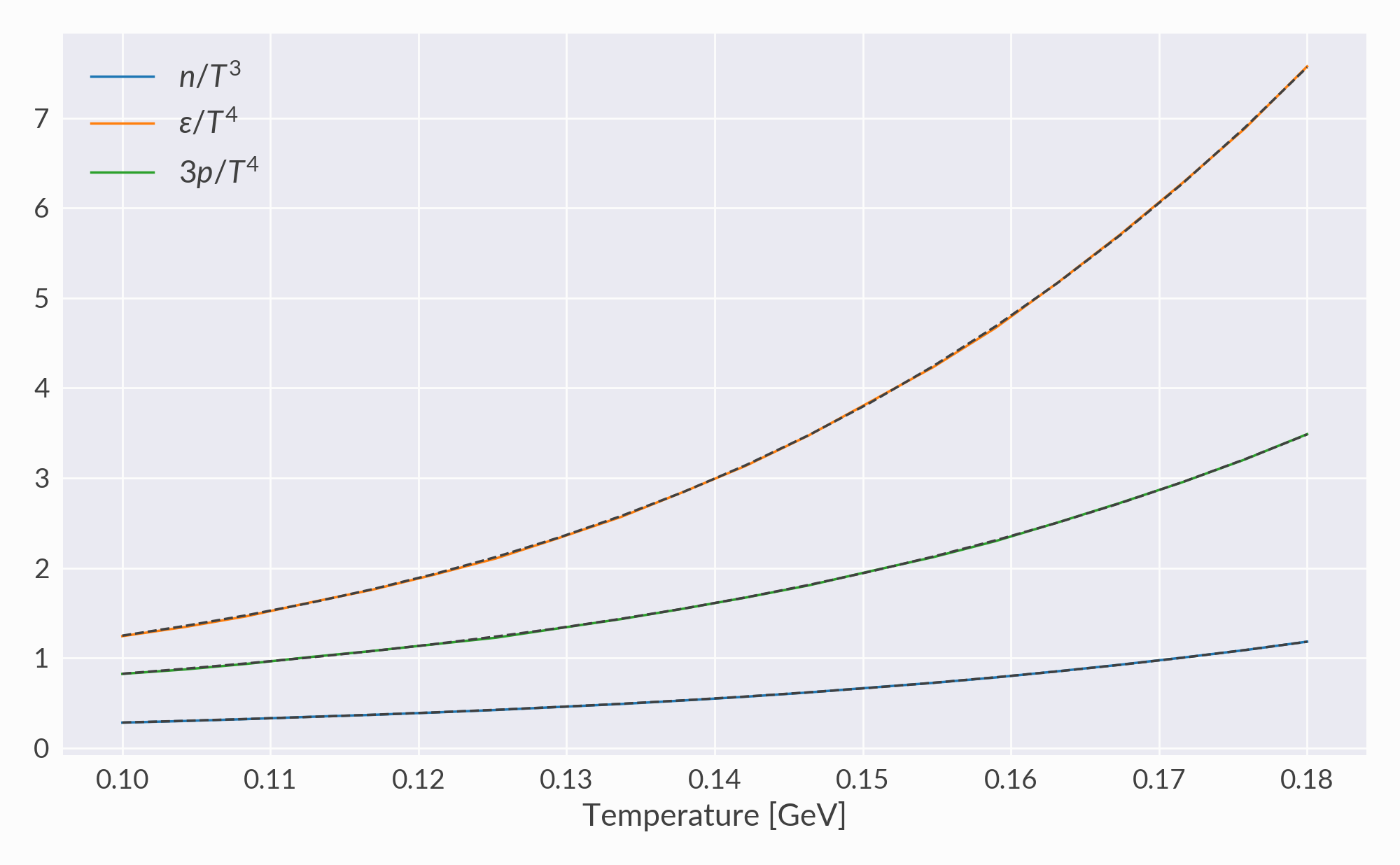
Equation of state
Comparison of thermodynamic quantities from phase-space integrals (grey dashed lines) to averages over sampled particles (solid colored lines).
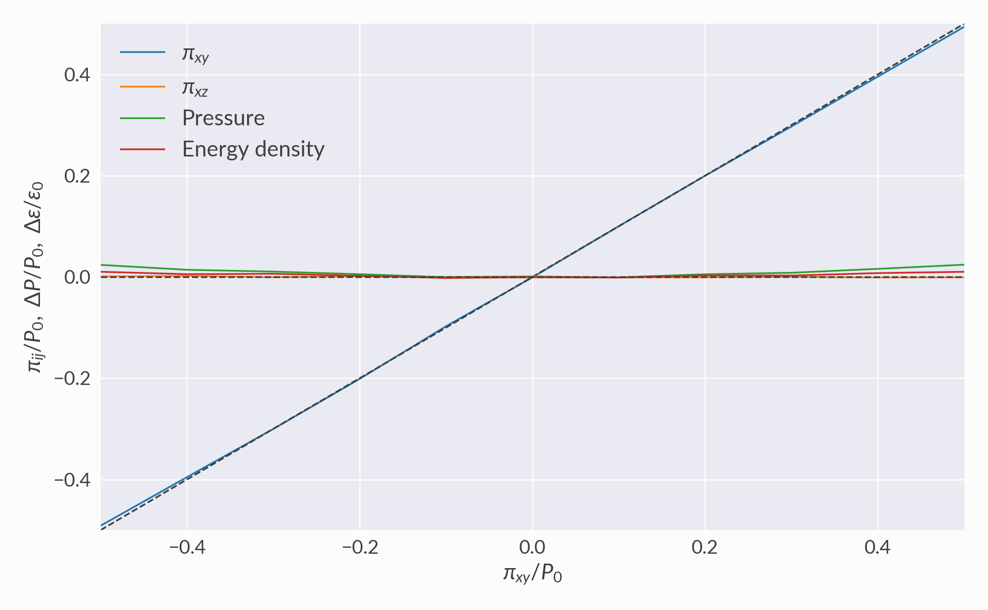
Shear viscous corrections
Verification that the desired shear tensor \(\pi^{\mu\nu}\) is reproduced. This test case checks that nonzero \(\pi^{xy}\) is reproduced without changing the equilibrium pressure or energy density. The algorithm starts to break down at very large shear pressure.
The “shear and bulk” section below has additional checks.
Bulk viscous corrections
Effect of bulk viscosity on thermodynamic quantities and momentum distributions.
The total pressure is the sum of the equilibrium and bulk pressures: \(P = P_0 + \Pi\). In order to satisfy continuity of the stress-energy tensor, sampled particles must reproduce the total pressure without changing the equilibrium energy density; this is achieved by parametrically rescaling overall particle production and momentum depending on the bulk pressure. This works for negative bulk pressure all the way down to zero total pressure, but for positive bulk pressure, the necessary momentum scale factor diverges as the total pressure approaches twice the equilibrium pressure. The momentum scale is therefore restricted to a reasonable maximum (3) which effectively limits the positive bulk pressure to around 70% of the equilibrium pressure, depending on the hadron gas temperature and composition.
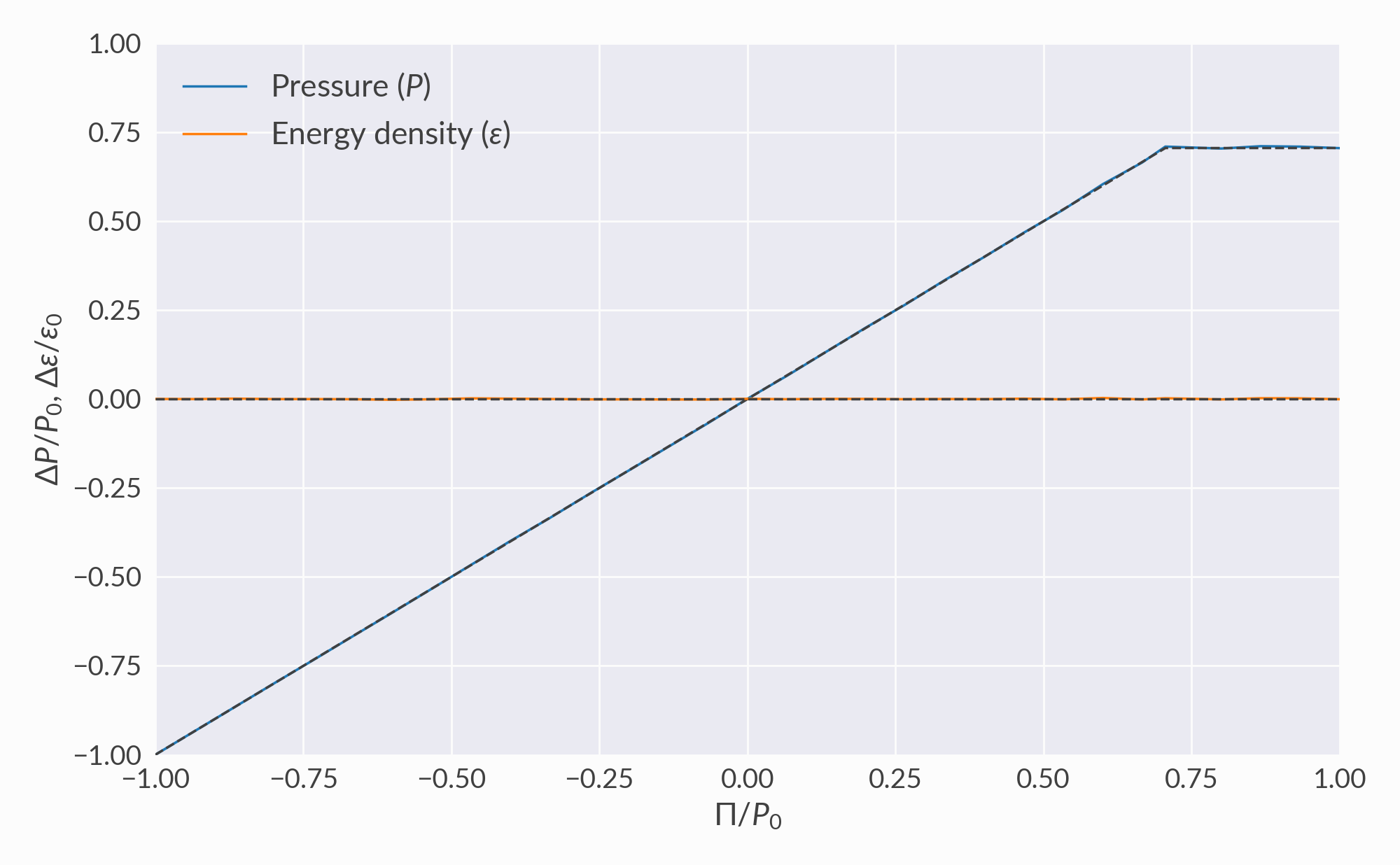
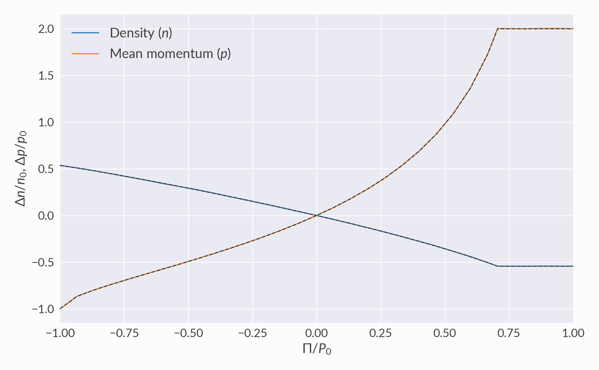
Most quantities are plotted as the relative change to their equilibrium values vs. the relative bulk pressure \(\Pi/P_0\). Colored lines are from samples and dashed lines are calculated.
Pressure and energy density
Bulk pressure changes the effective pressure without changing the energy density.
Particle density and momentum
The changes in particle density and mean momentum necessary to achieve the target pressure and energy density.
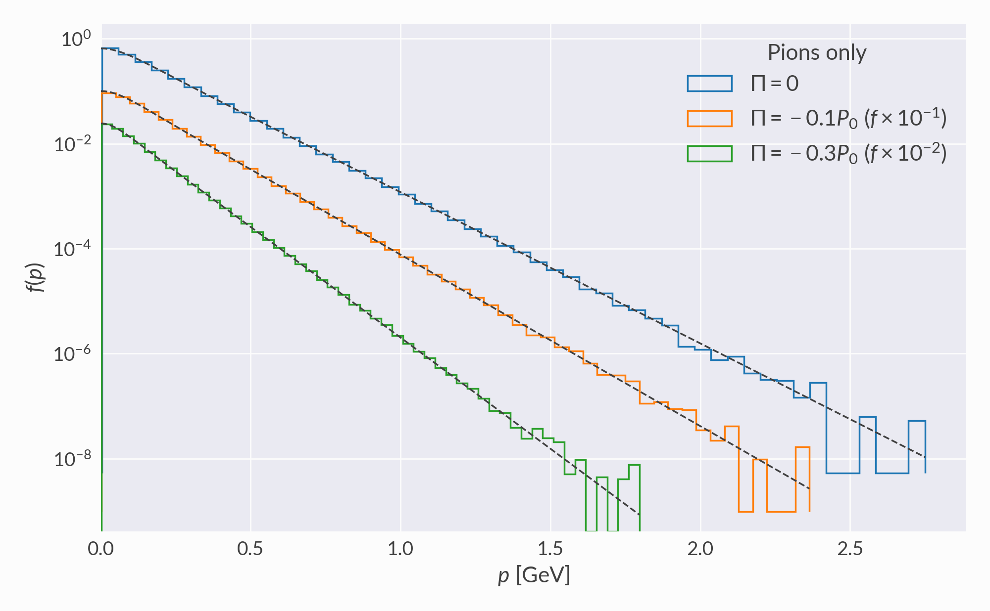
Distribution functions
Pion distribution functions \(f(p)\) for different bulk pressures. Colored histograms are samples; dashed lines are target distributions with rescaled momentum, \(f(\lambda p)\).
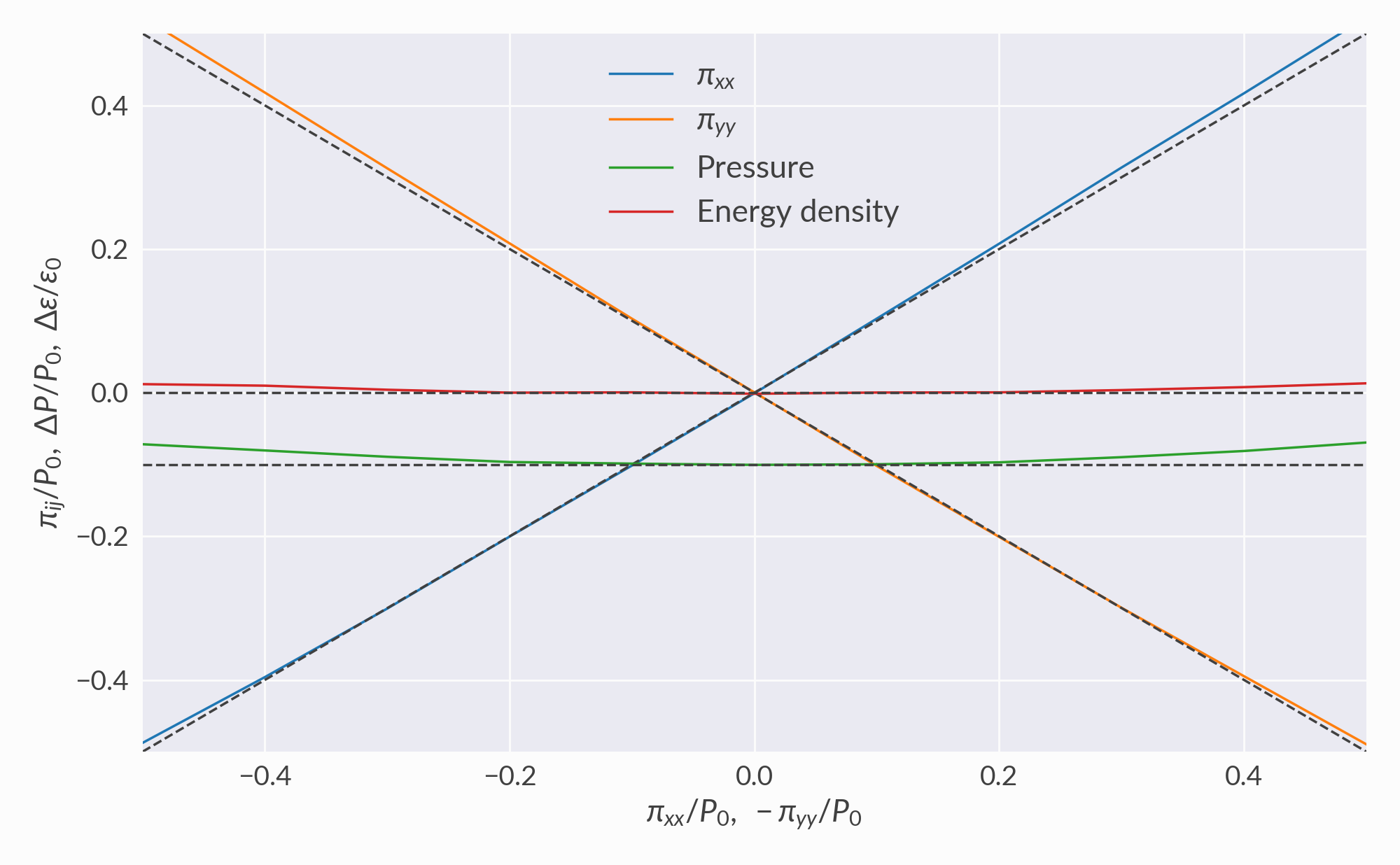
Shear and bulk
Shear tensor with \(\pi^{xx} = -\pi^{yy}\) and all other components zero, and bulk pressure fixed at \(\Pi = -0.1P_0\). This is a very difficult test case but the algorithm remains accurate for small to moderate viscous pressure.
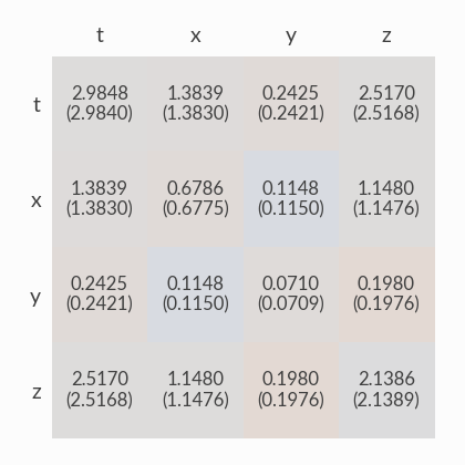
Stress energy tensor
Verification that the sampling algorithm reproduces the complete stress-energy tensor \(T^{\mu\nu}\) from hydrodynamics, including any viscous corrections.
For each of the following, the flow velocity and viscous pressures are chosen randomly, particles are sampled, and the effective stress-energy tensor is computed by summing over the sampled particles. The sampled tensor is then compared to the expectation from hydro.
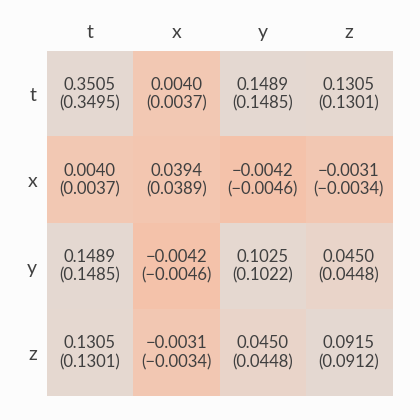
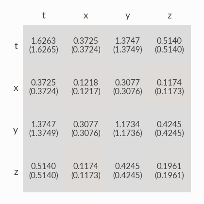
In the heatmap cells, the first number is sampled value for the given component of the tensor and the second number (in parentheses) is the expected value from hydro. Cells are color-coded, where grey indicates perfect agreement, red indicates that the sampled value is large, and blue too small. Some disagreement is expected due to statistical fluctuations from finite numbers of particles.
Before each heatmap, the randomly chosen velocity and viscous pressures are listed. The overall magnitude of shear pressure is quantified by the Lorentz scalar “pirel” = \(\sqrt{\pi^{\mu\nu}\pi_{\mu\nu}/(e^2 + 3P_0^2)}\).
v = (0.023, 0.380, 0.332), pirel = 0.060, Pi/P0 = 0.037
v = (0.221, 0.826, 0.308), pirel = 0.017, Pi/P0 = −0.104
v = (0.458, 0.081, 0.827), pirel = 0.040, Pi/P0 = 0.197